Latest Year Analysis
Meteorological Year
(Annual values correspond to the period from December to November)
2024
|
|
TEMPERATURE ANOMALY
|
Minimum Temperature
|
Mean Temperature
|
Maximum Temperature
|
|
Solar Year
(Annual values correspond to the period from January to December)
2024
|
|
TEMPERATURE ANOMALY
|
Minimum Temperature
|
Mean Temperature
|
Maximum Temperature
|
|
Back to Top
Year-to-date Analysis
Meteorological Year
(Annual values correspond to the period from December to November)
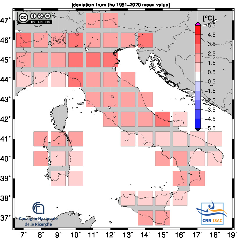
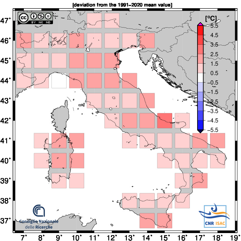
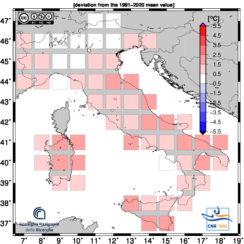
DECEMBER - AUGUST 2025
|
|
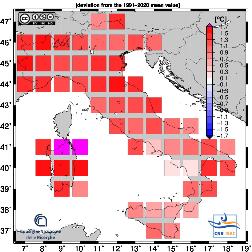
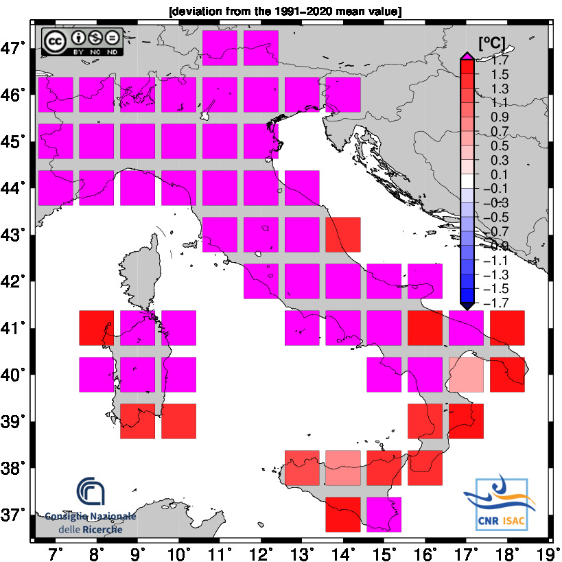
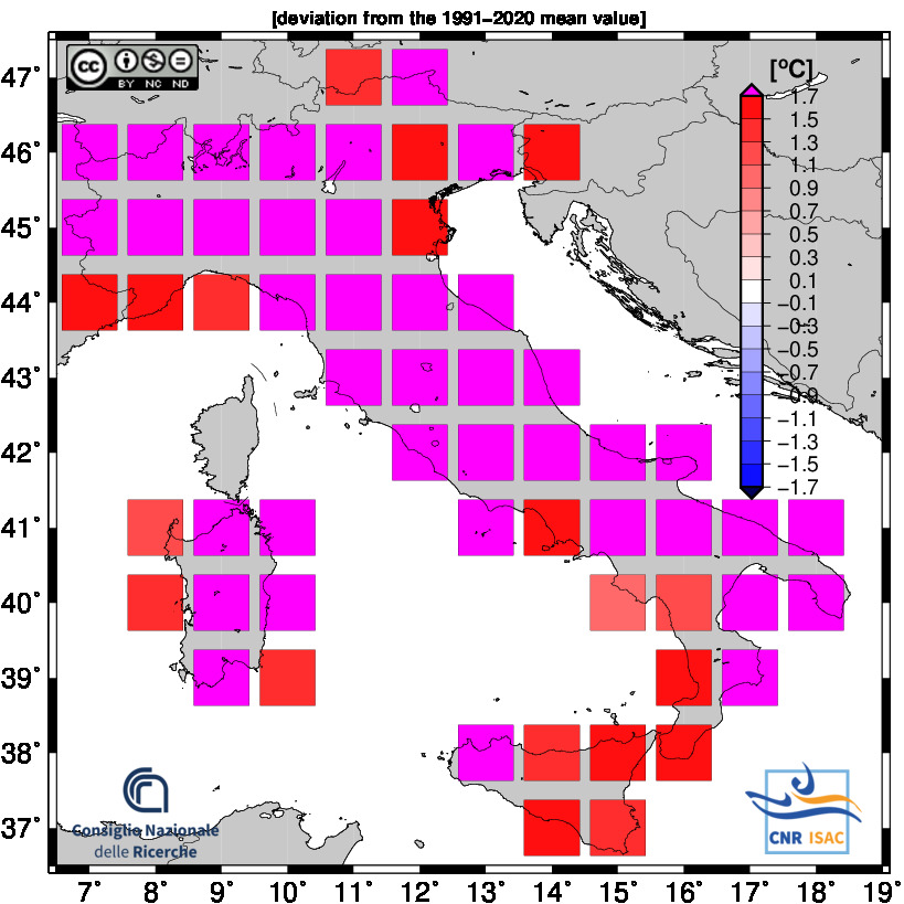
TEMPERATURE ANOMALY
|
Minimum Temperature

|
Mean Temperature

|
Maximum Temperature

|
|
Solar Year
(Annual values correspond to the period from January to December)
JANUARY - AUGUST 2025
|
|
TEMPERATURE ANOMALY
|
Minimum Temperature
|
Mean Temperature

|
Maximum Temperature
|
|
Back to Top
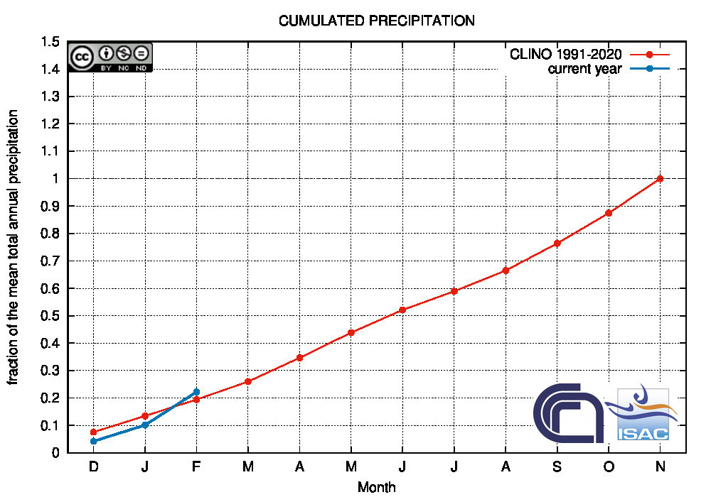
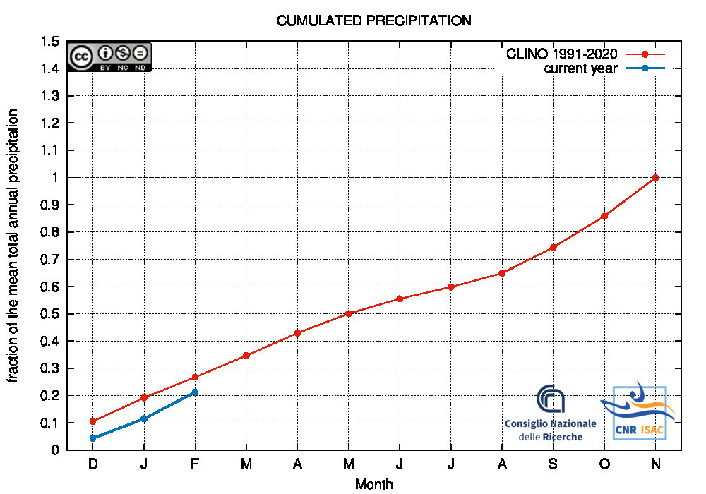
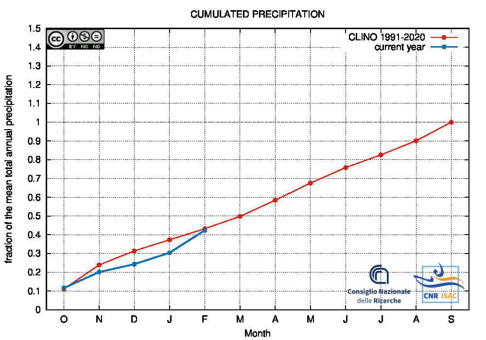
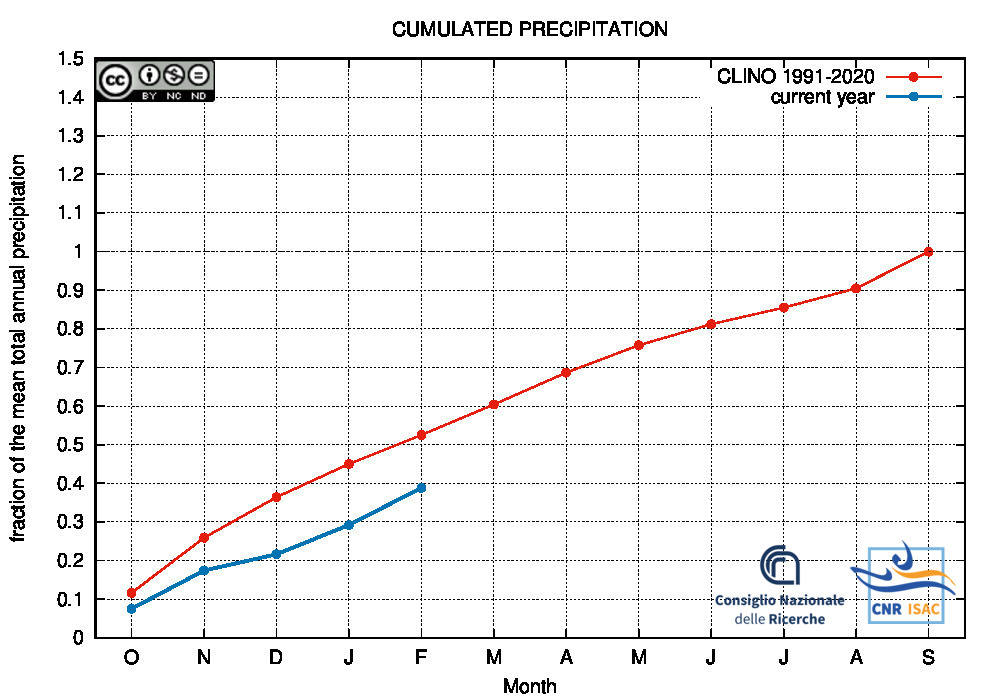
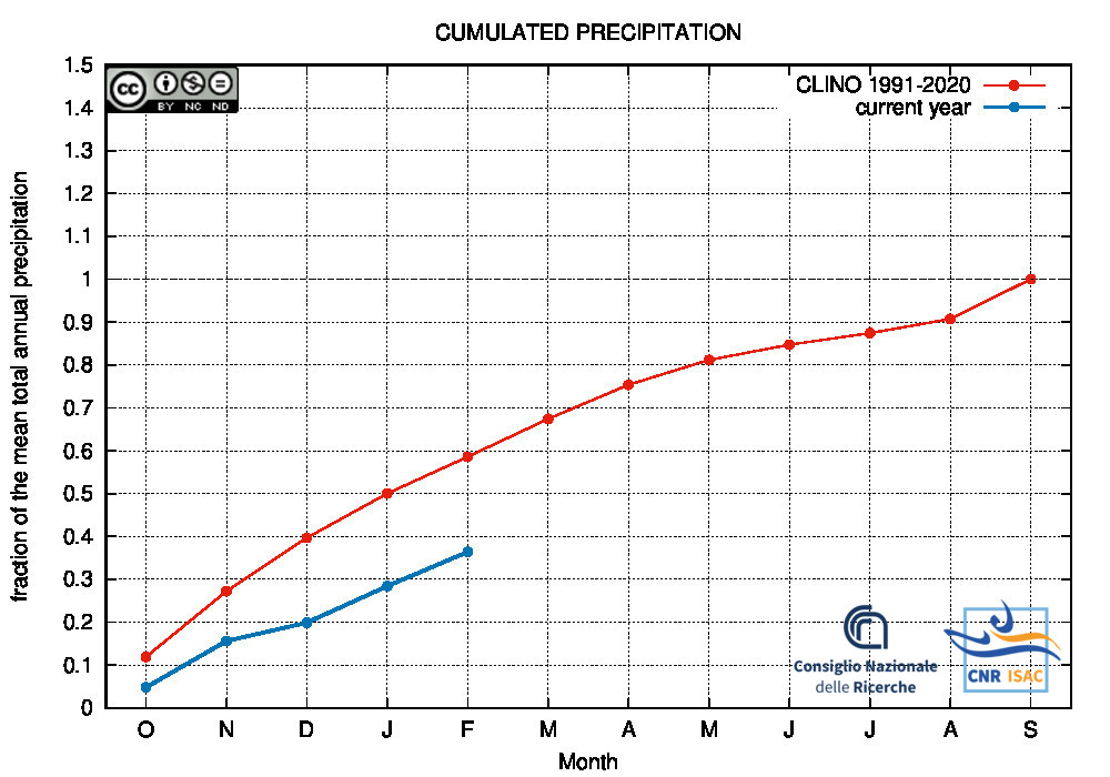
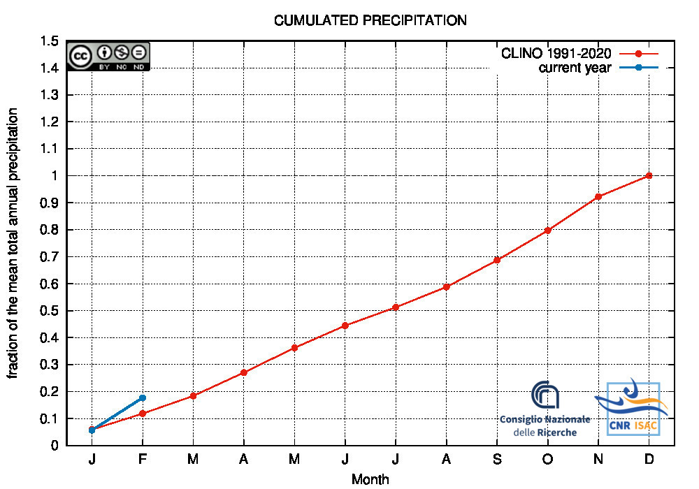
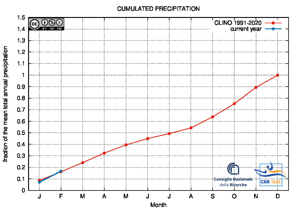
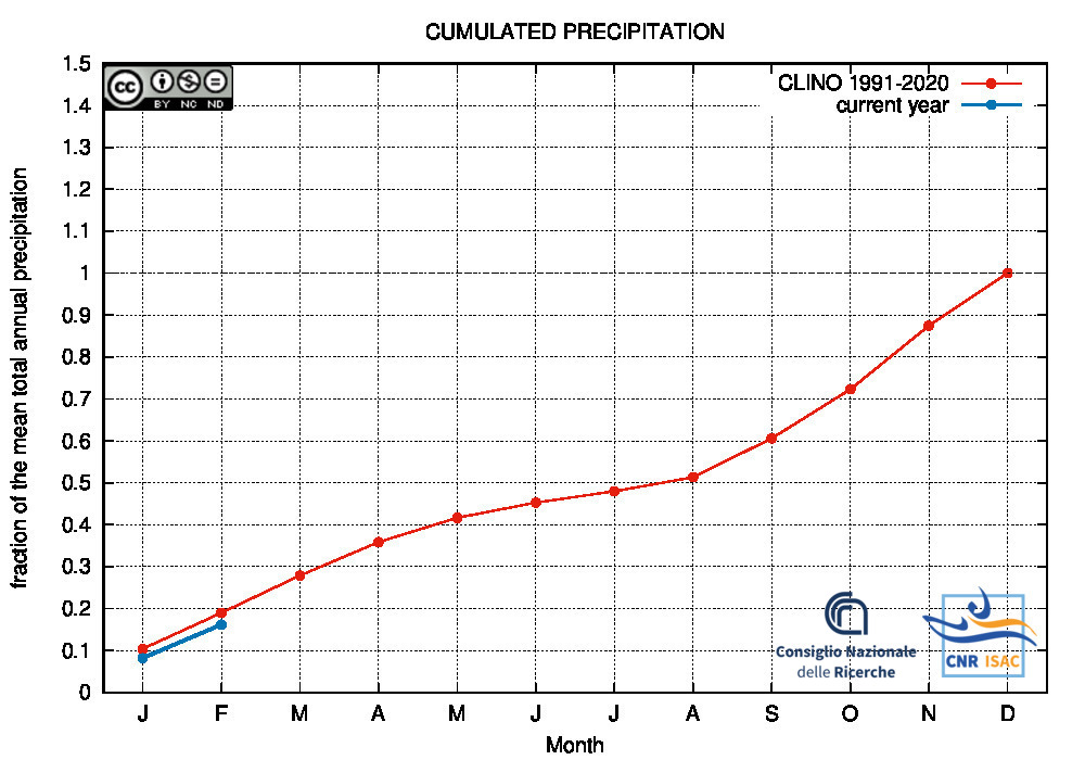
Drought/Wetness Monitoring
Comparison of the cumulated precipitation along the current year with the climatological cumulated values (reference period 1991-2020)
METEOROLOGICAL YEAR
2025
(December to November)
Northern Italy
|
Italy
|
Southern Italy

|
HYDROLOGICAL YEAR
2025
(October to September)
Northern Italy
|
Italy
|
Southern Italy
|
SOLAR YEAR
2025
(January to December)
Northern Italy
|
Italy
|
Southern Italy
|
Back to Top
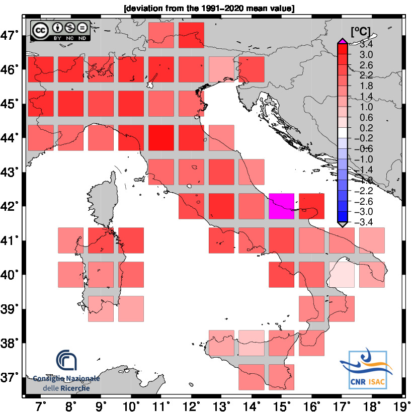
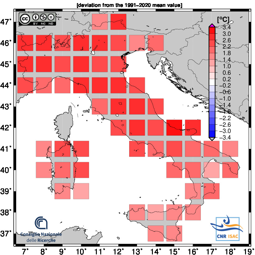
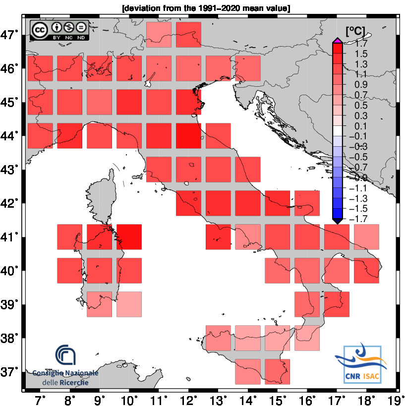
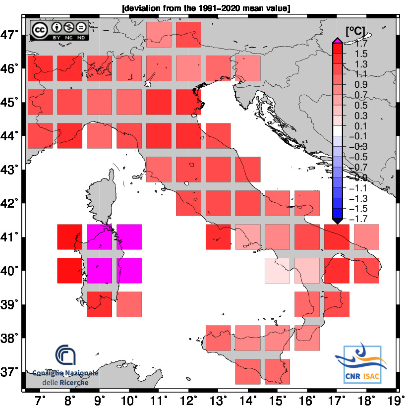
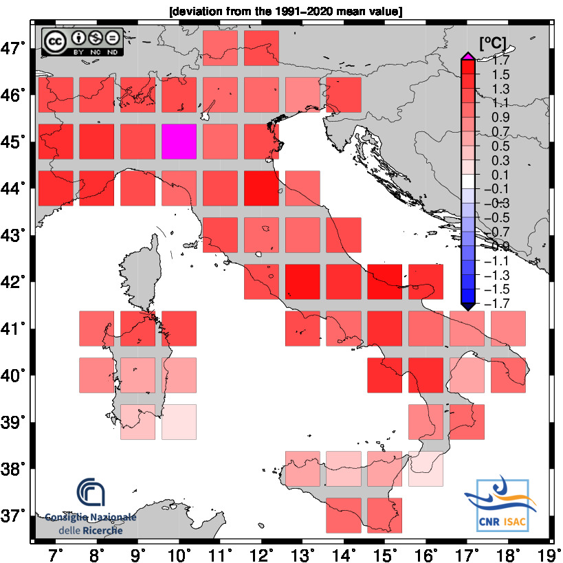
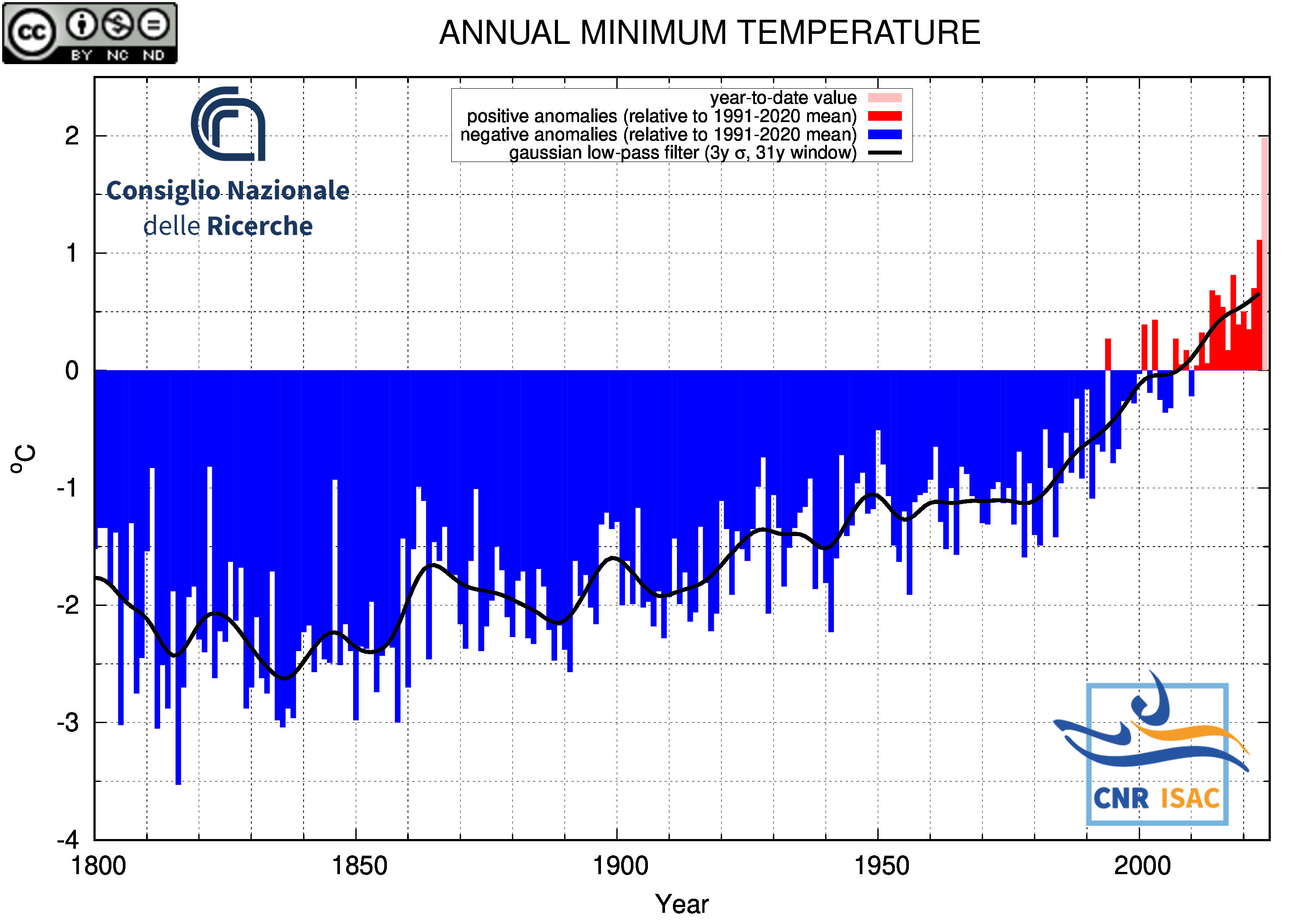
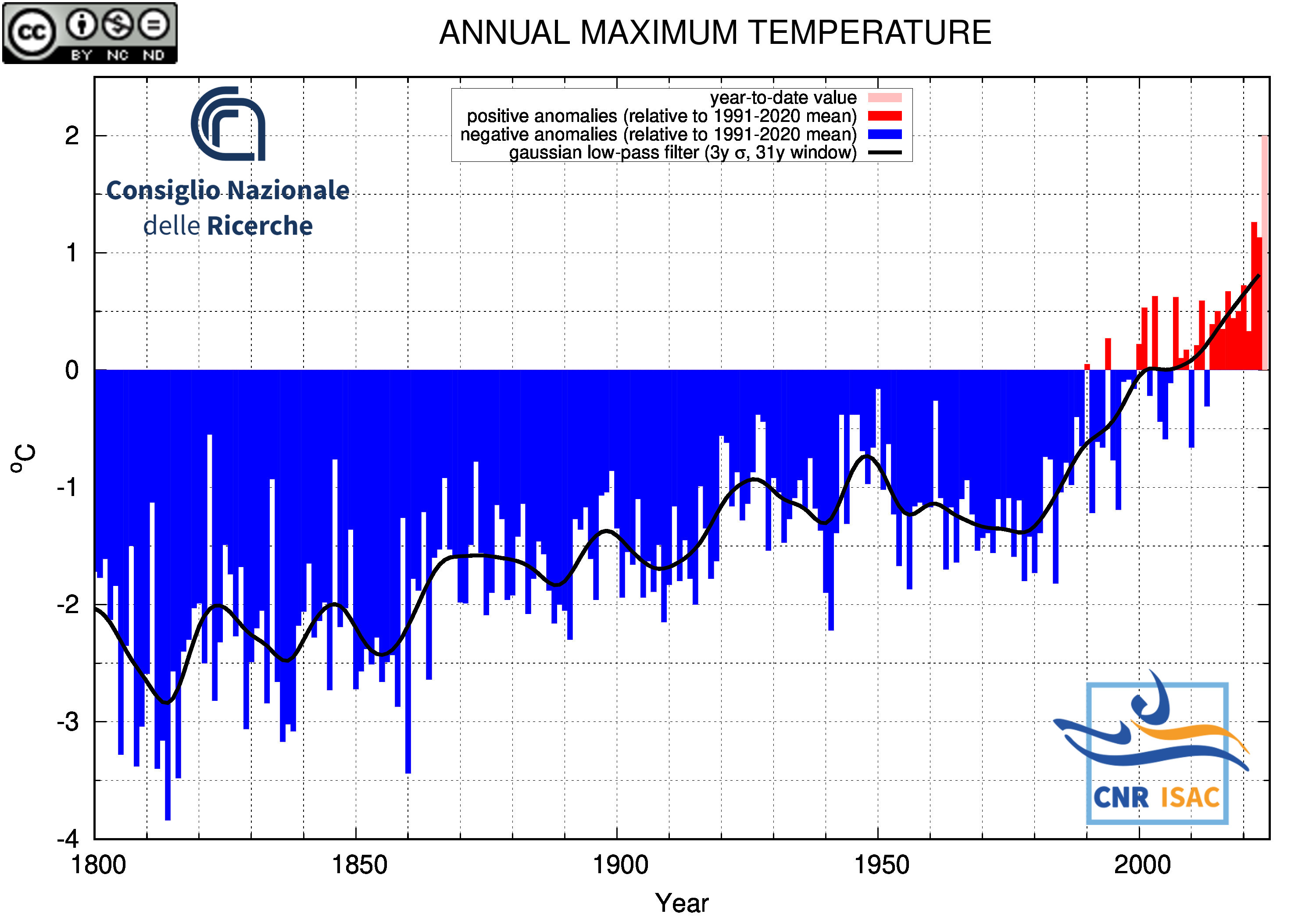
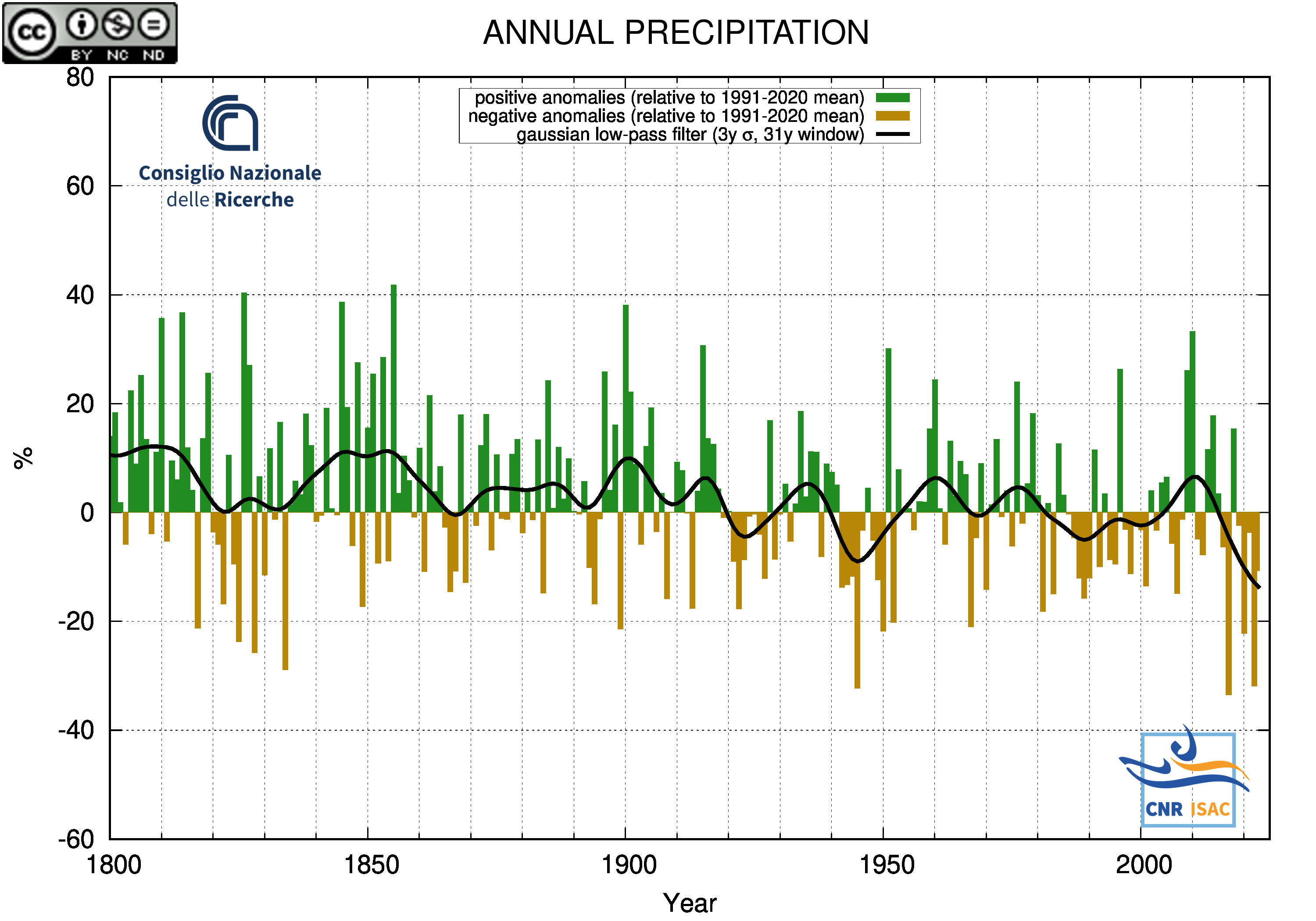
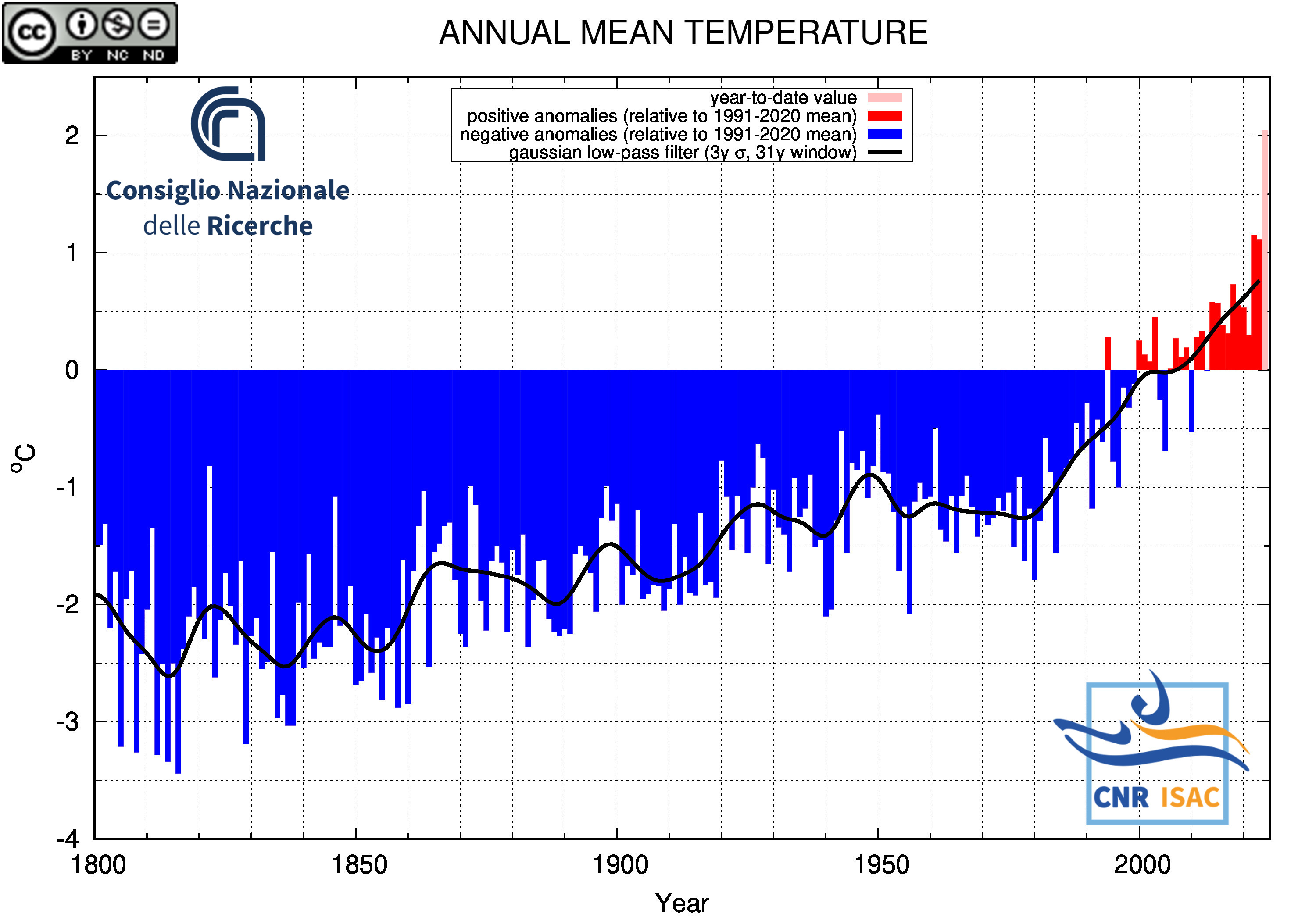
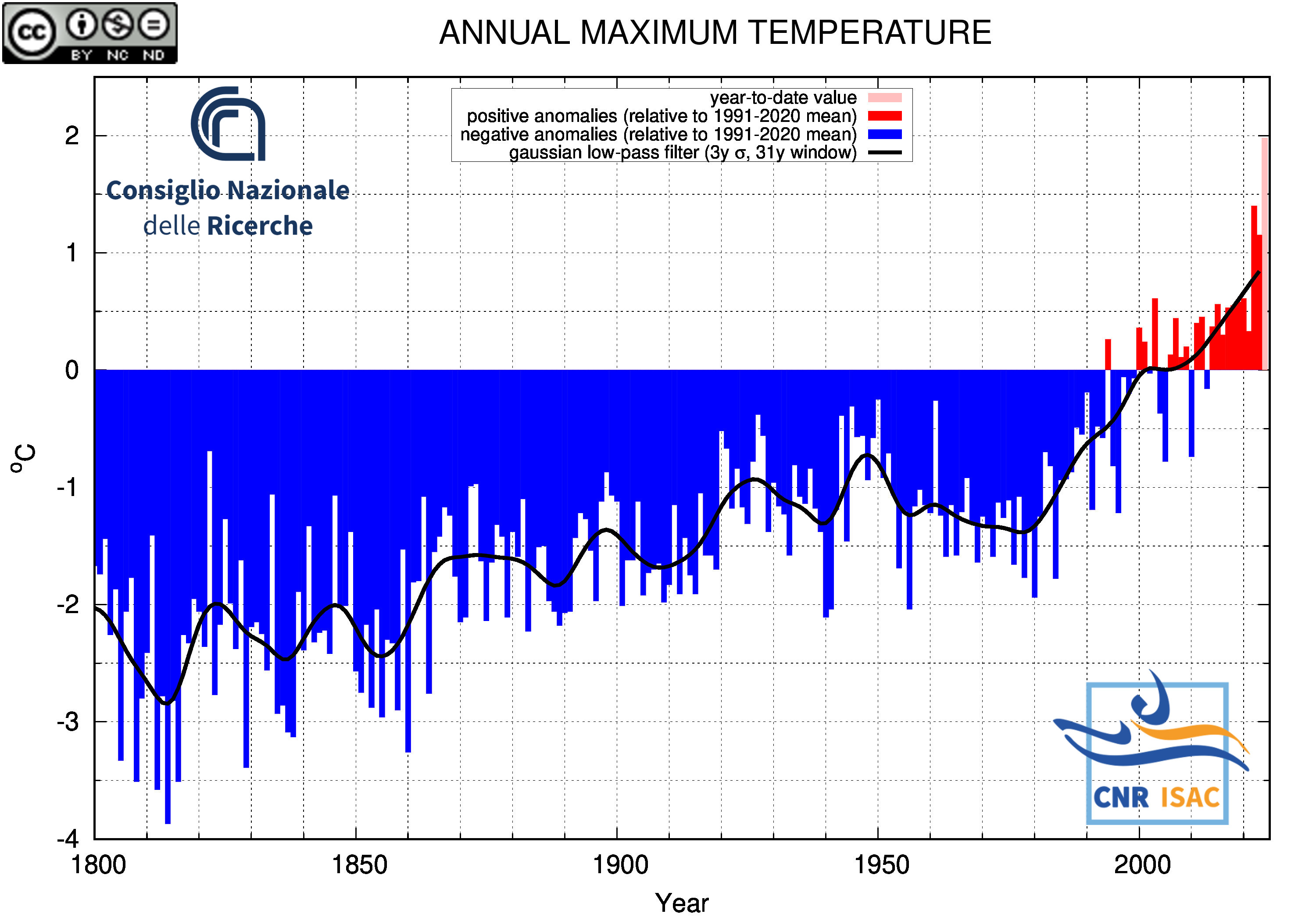
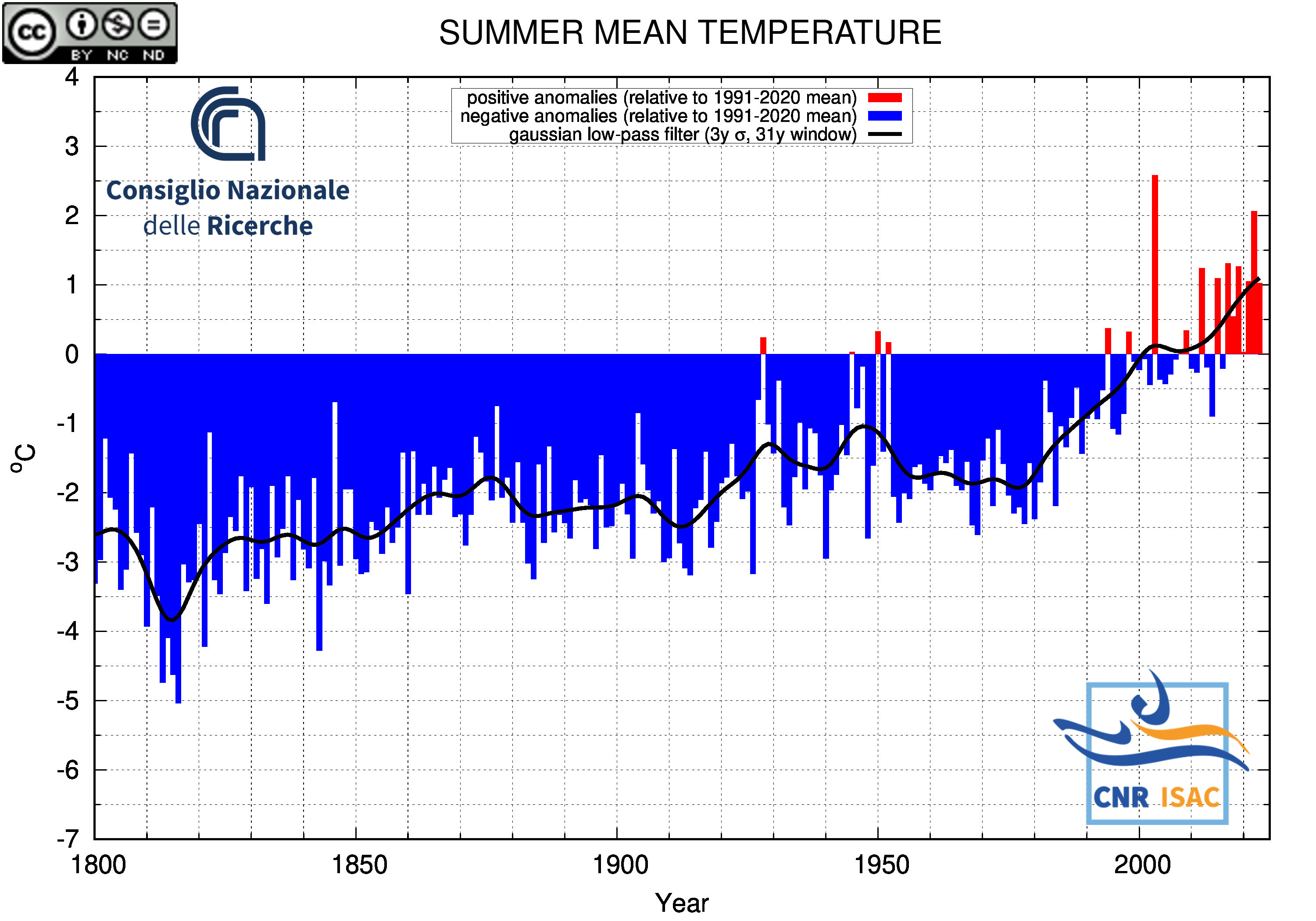
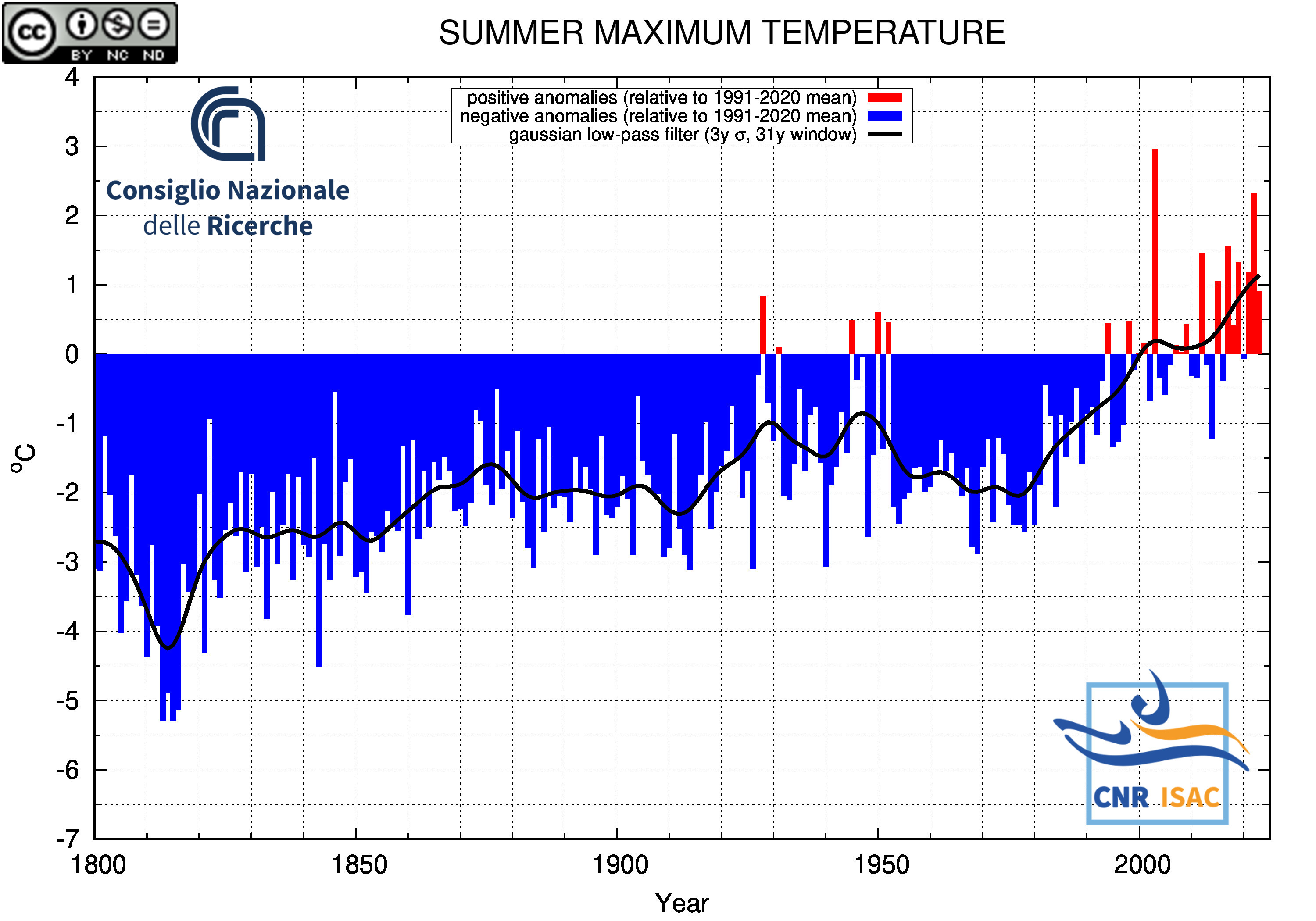
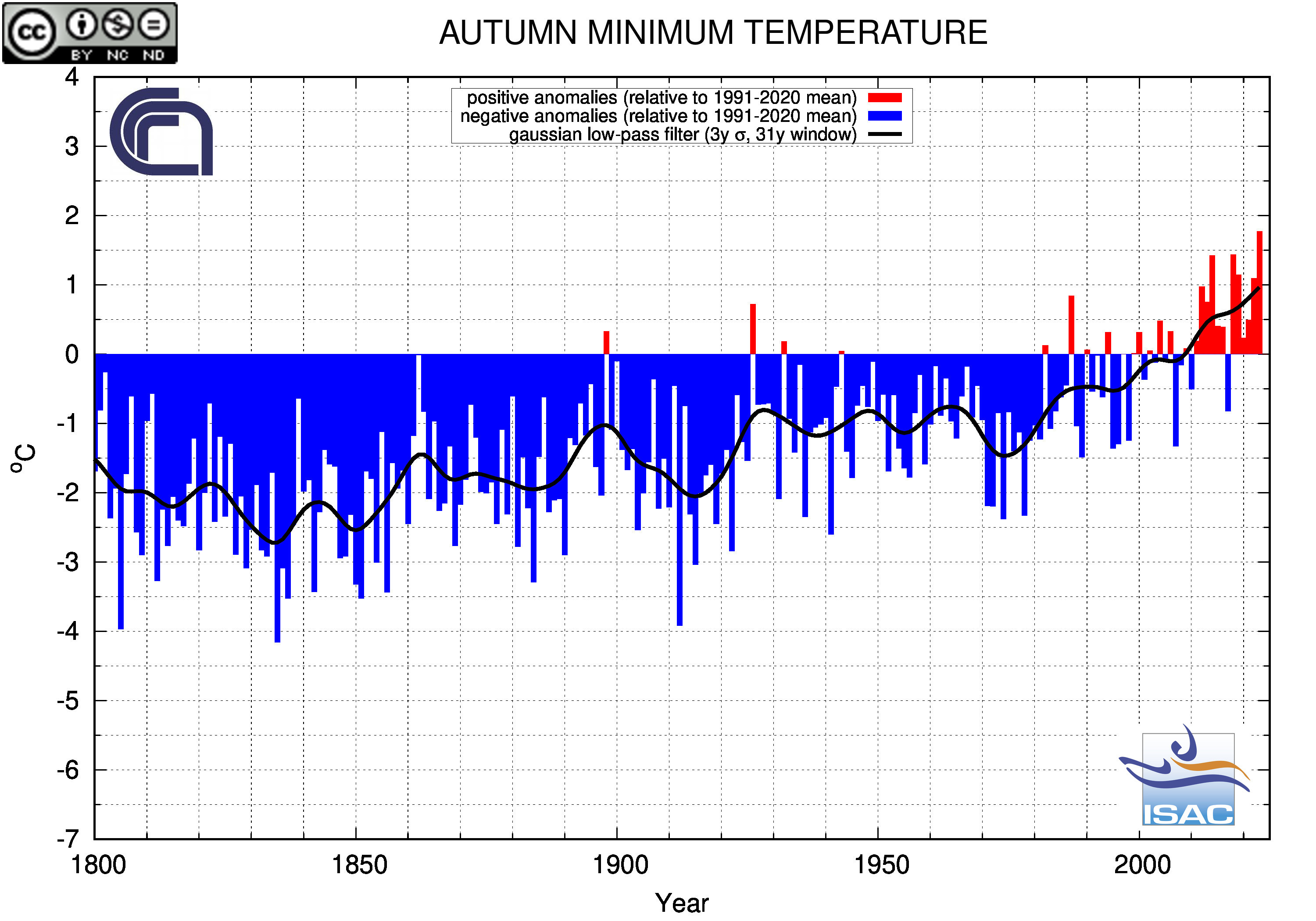
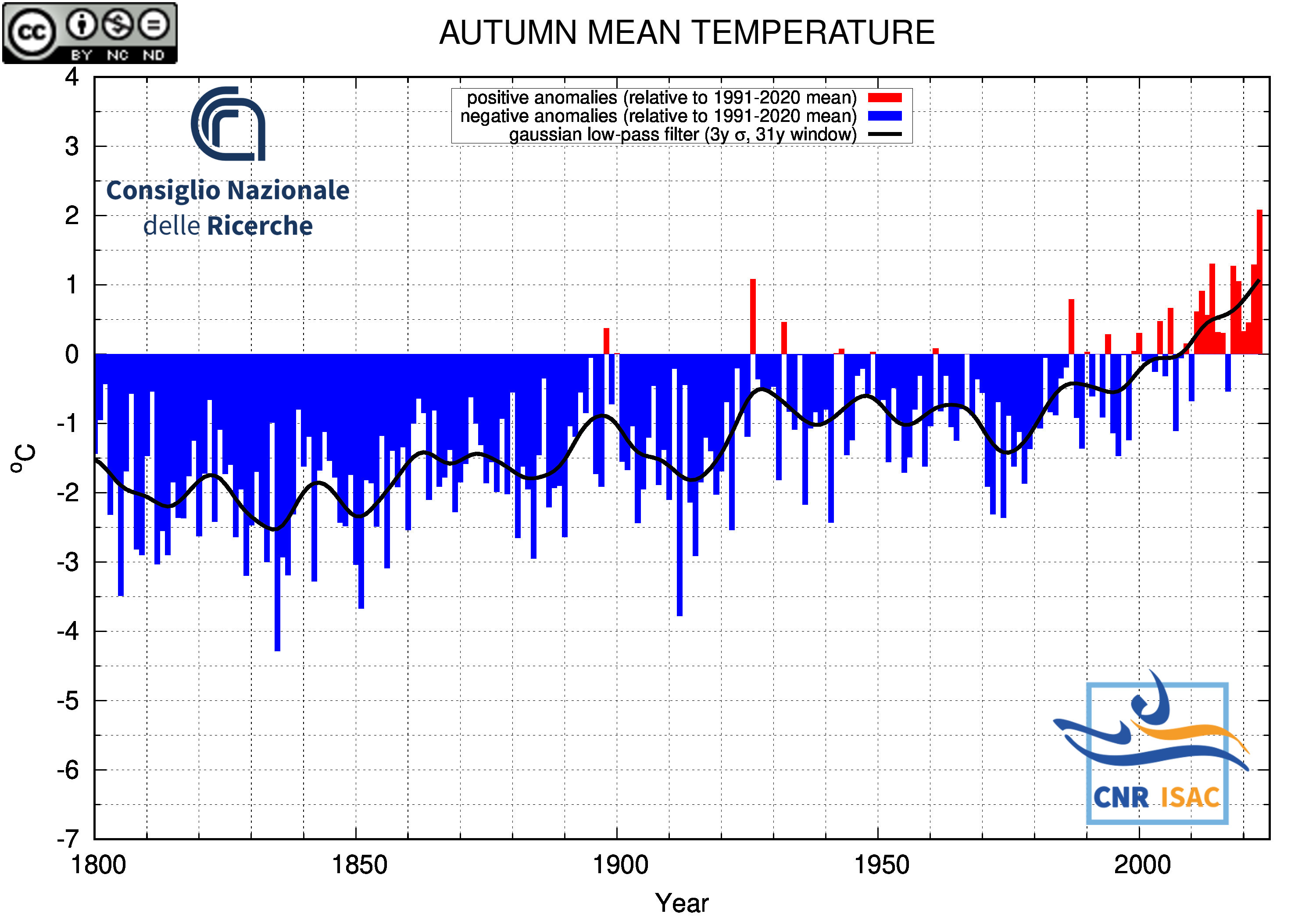
Long-Term Analysis
Italian Mean Temperature and Precipitation Series
(deviation from the 1991-2020 mean)
METEOROLOGICAL YEAR
(December to November)
|
TEMPERATURE ANOMALY
|
PRECIPITATION ANOMALY
|
Minimum Temperature
|
Mean Temperature

|
Maximum Temperature
|
|
|
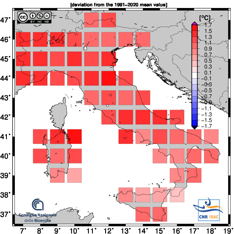
SOLAR YEAR
(January to December)
|
TEMPERATURE ANOMALY
|
PRECIPITATION ANOMALY
|
Minimum Temperature

|
Mean Temperature
|
Maximum Temperature
|
|

|
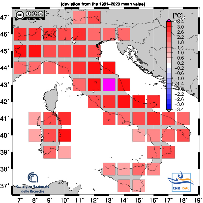
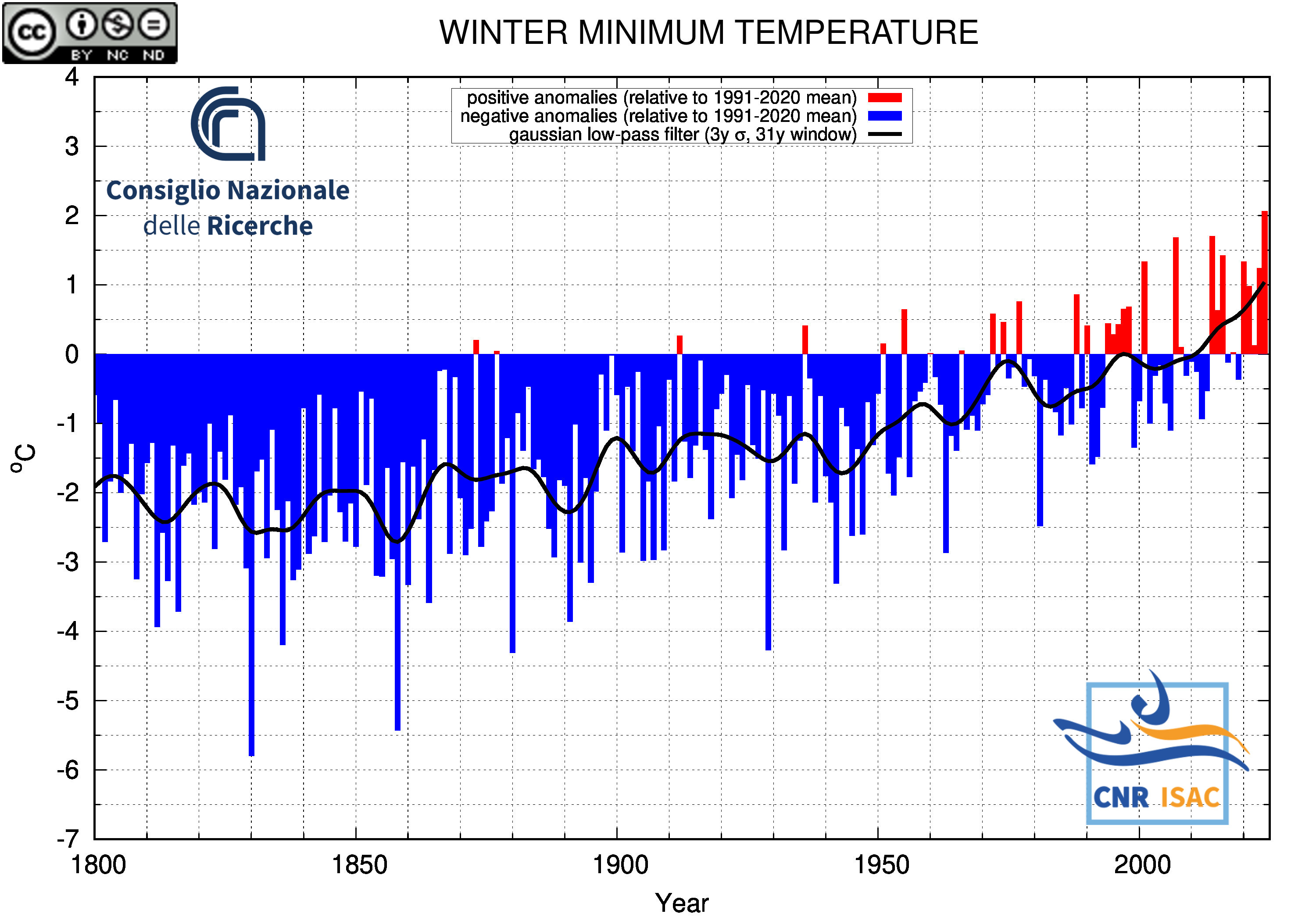
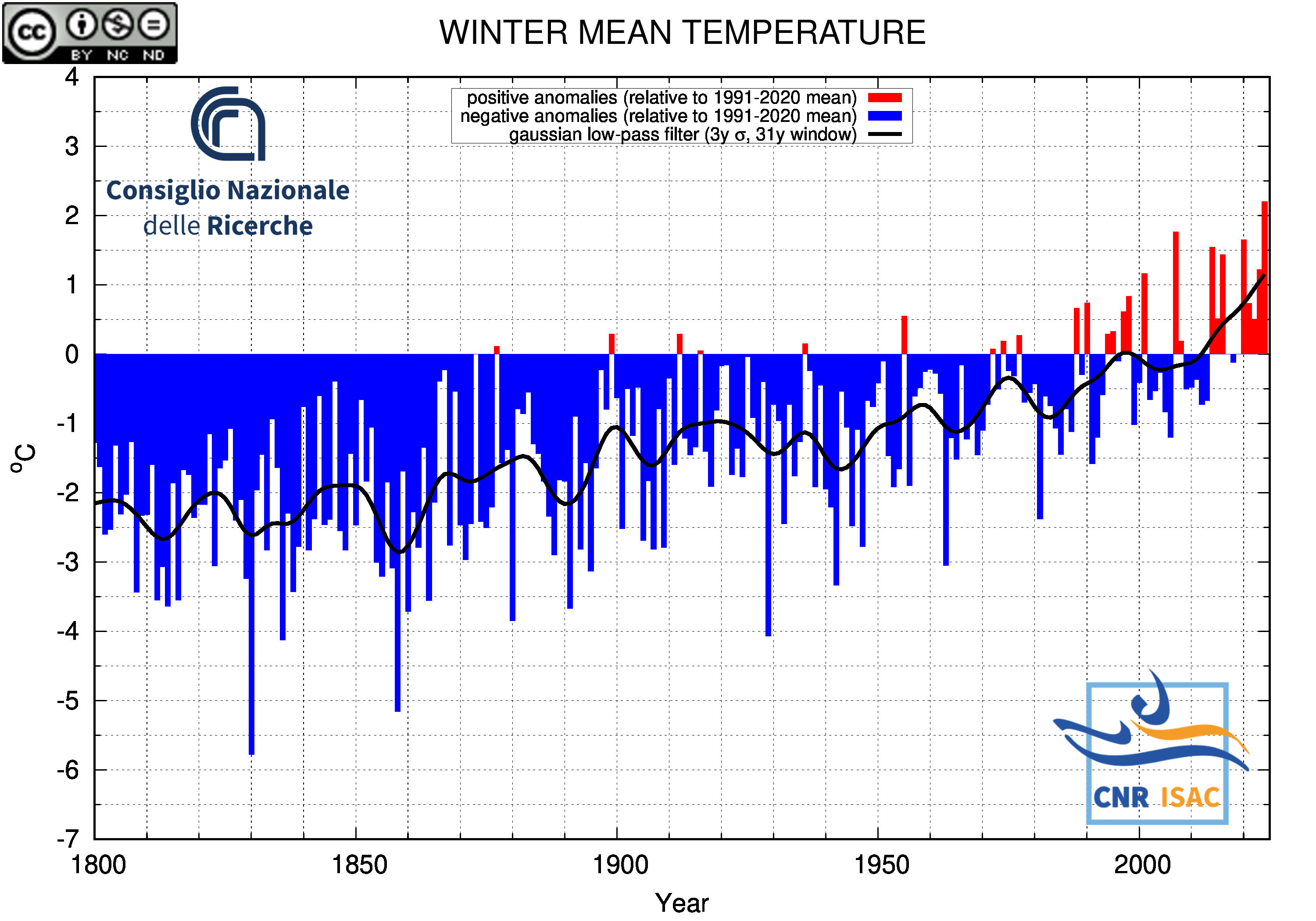
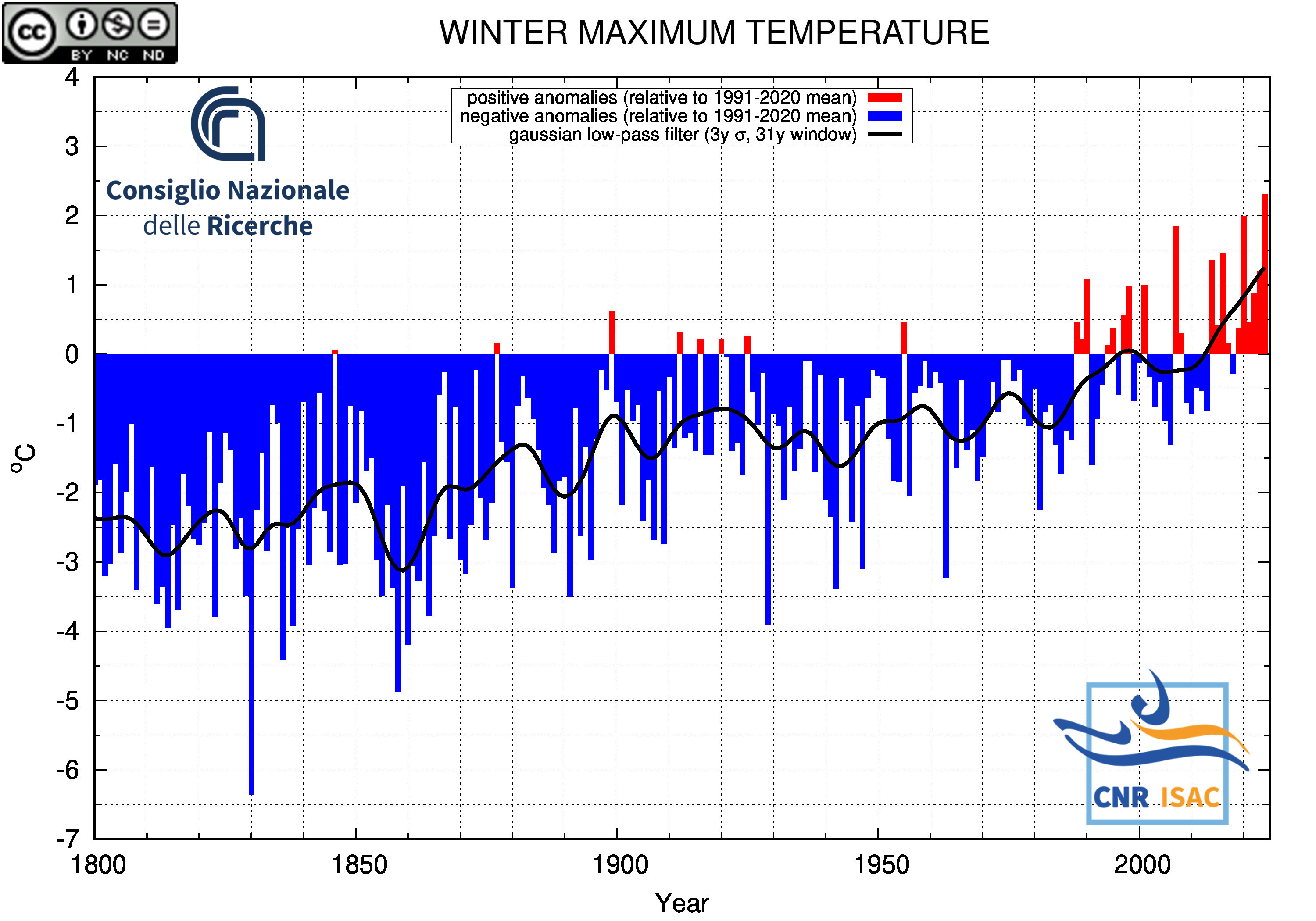
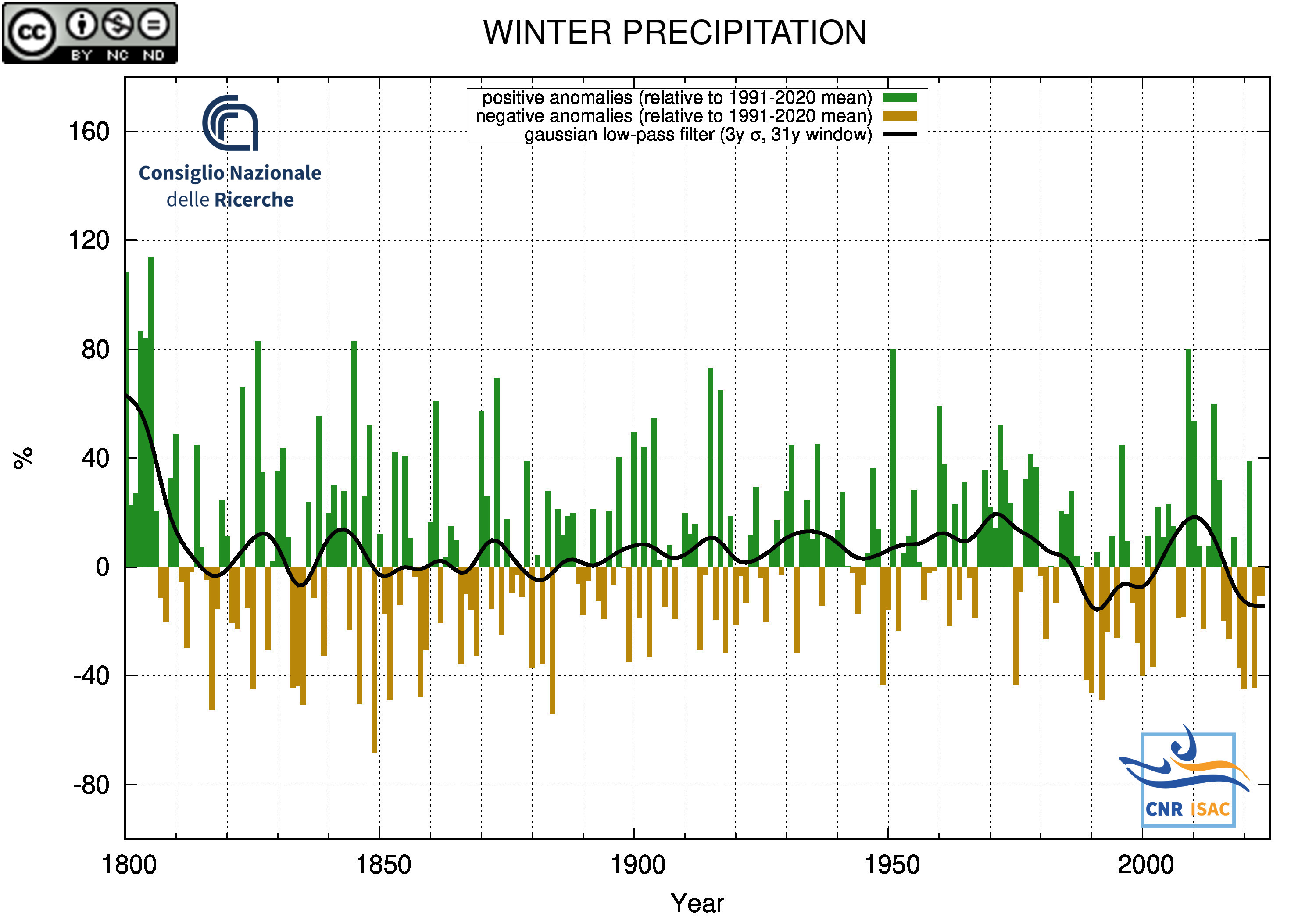
WINTER
(DJF)
|
TEMPERATURE ANOMALY
|
PRECIPITATION ANOMALY
|
Minimum Temperature
|
Mean Temperature
|
Maximum Temperature
|
|
|
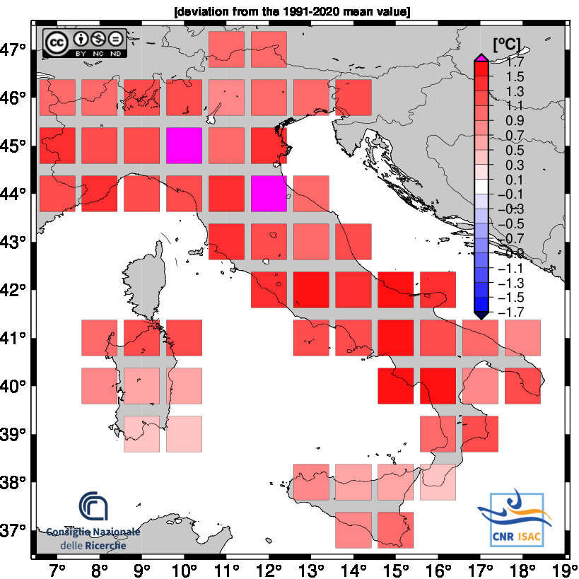
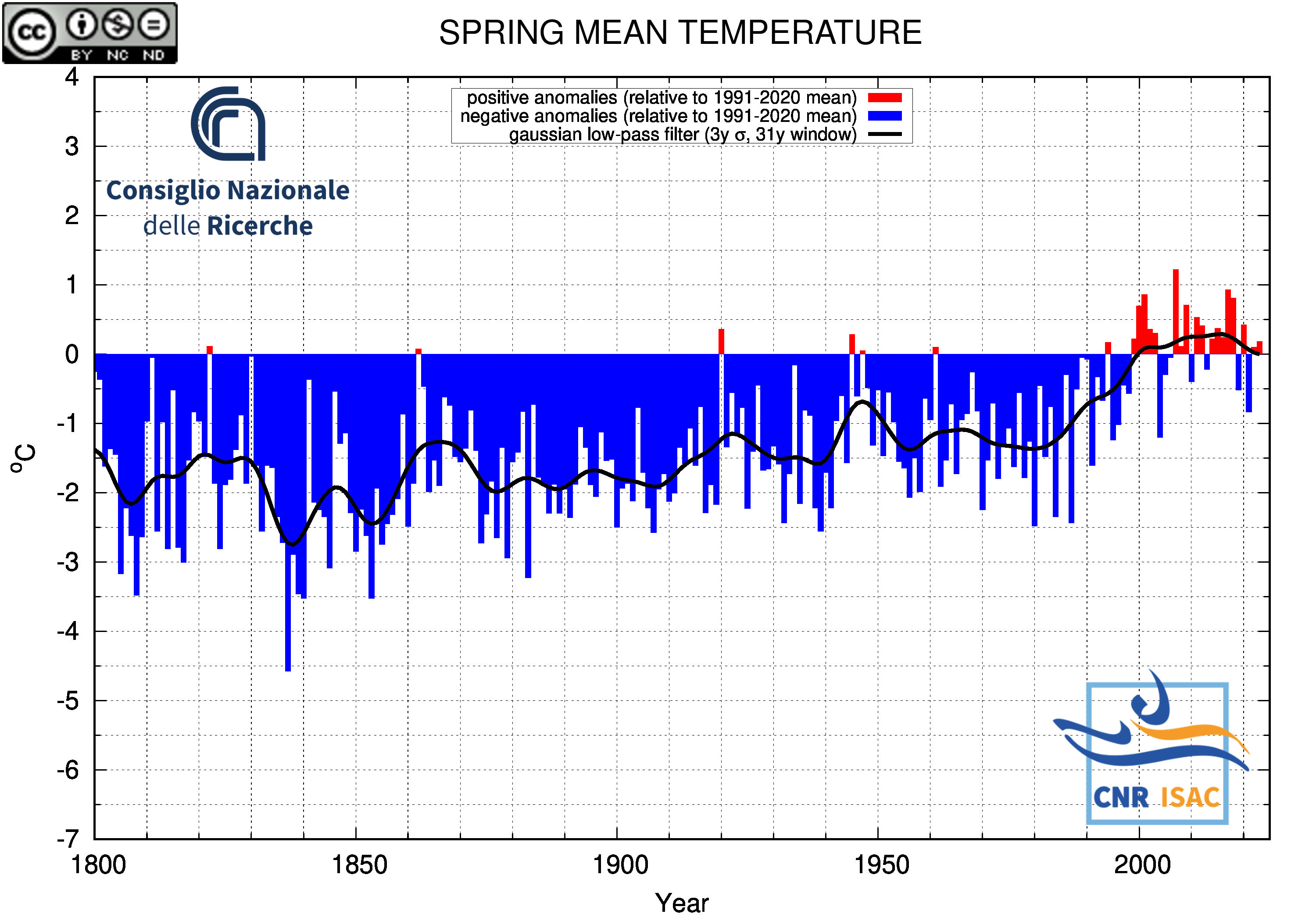
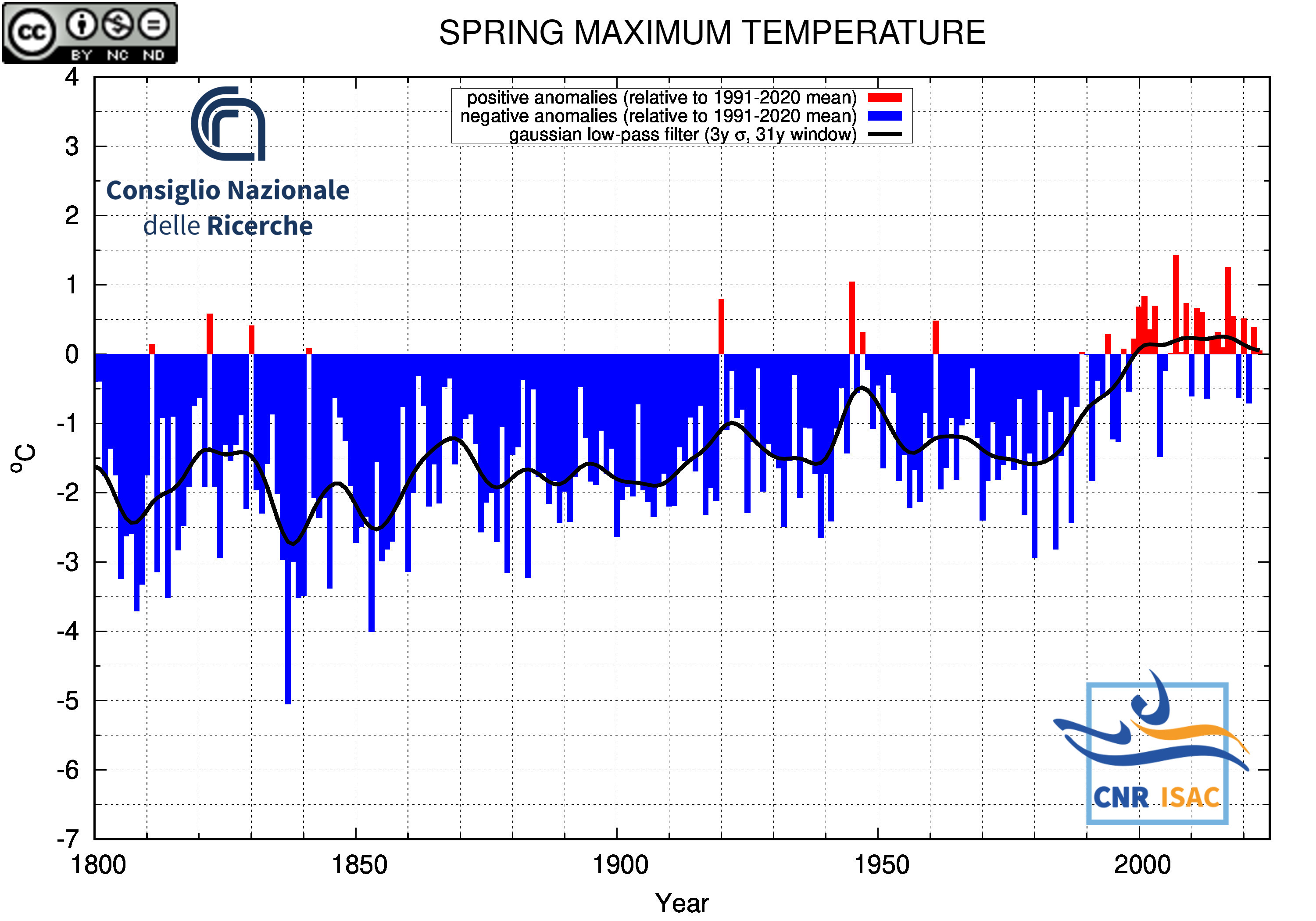
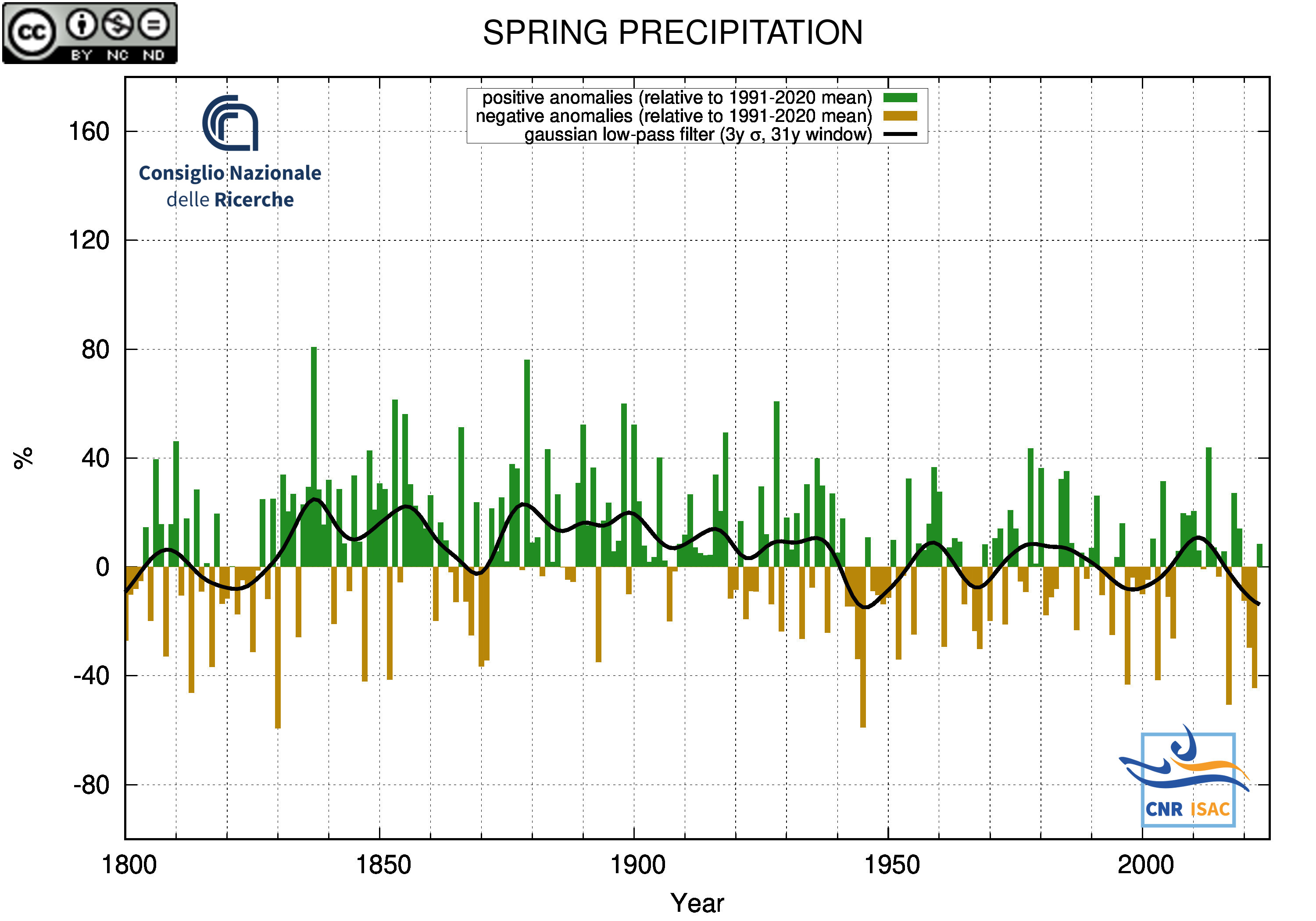
SPRING
(MAM)
|
TEMPERATURE ANOMALY
|
PRECIPITATION ANOMALY
|
Minimum Temperature

|
Mean Temperature
|
Maximum Temperature
|
|
|
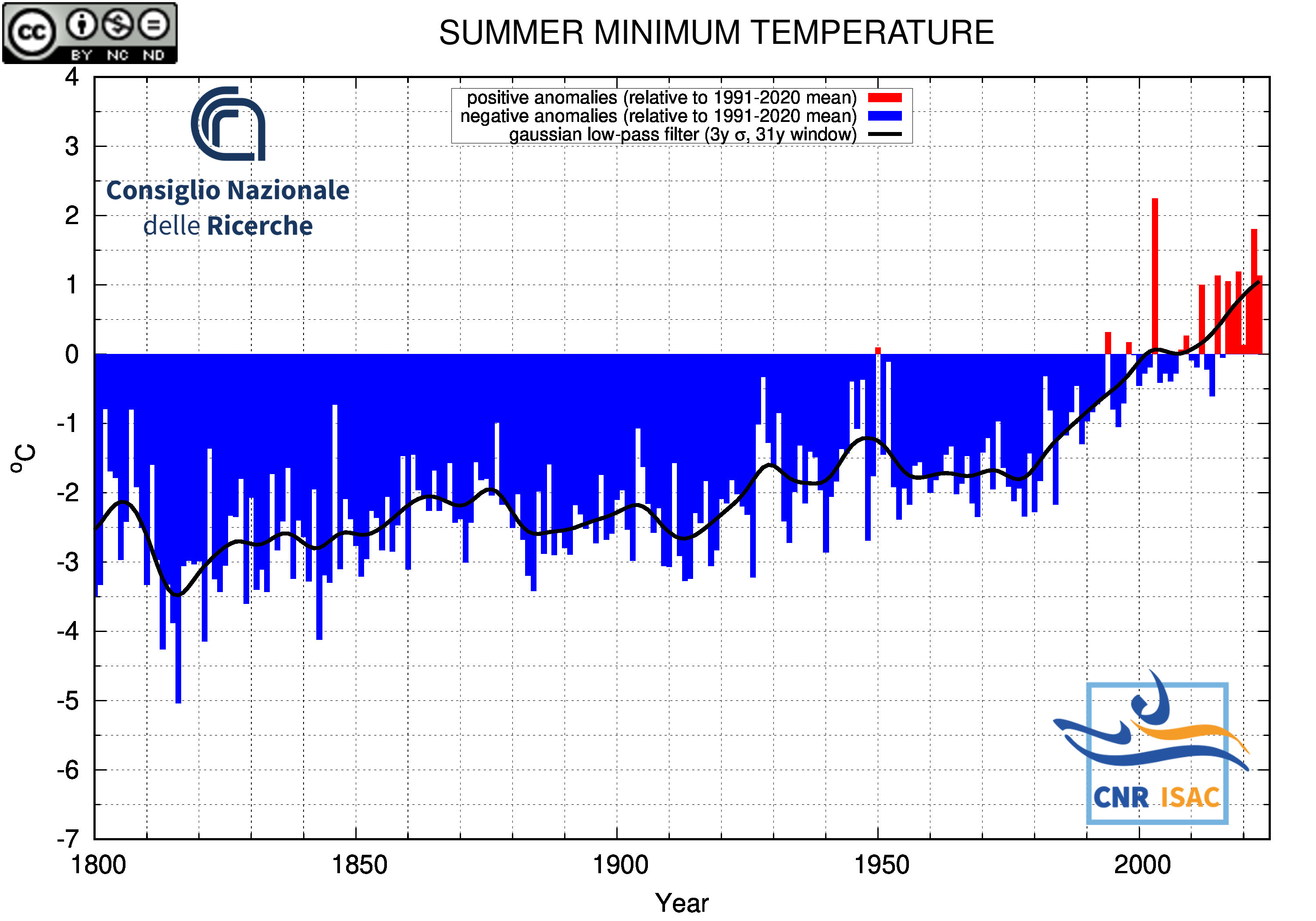
SUMMER
(JJA)
|
TEMPERATURE ANOMALY
|
PRECIPITATION ANOMALY
|
Minimum Temperature
|
Mean Temperature
|
Maximum Temperature
|
|

|
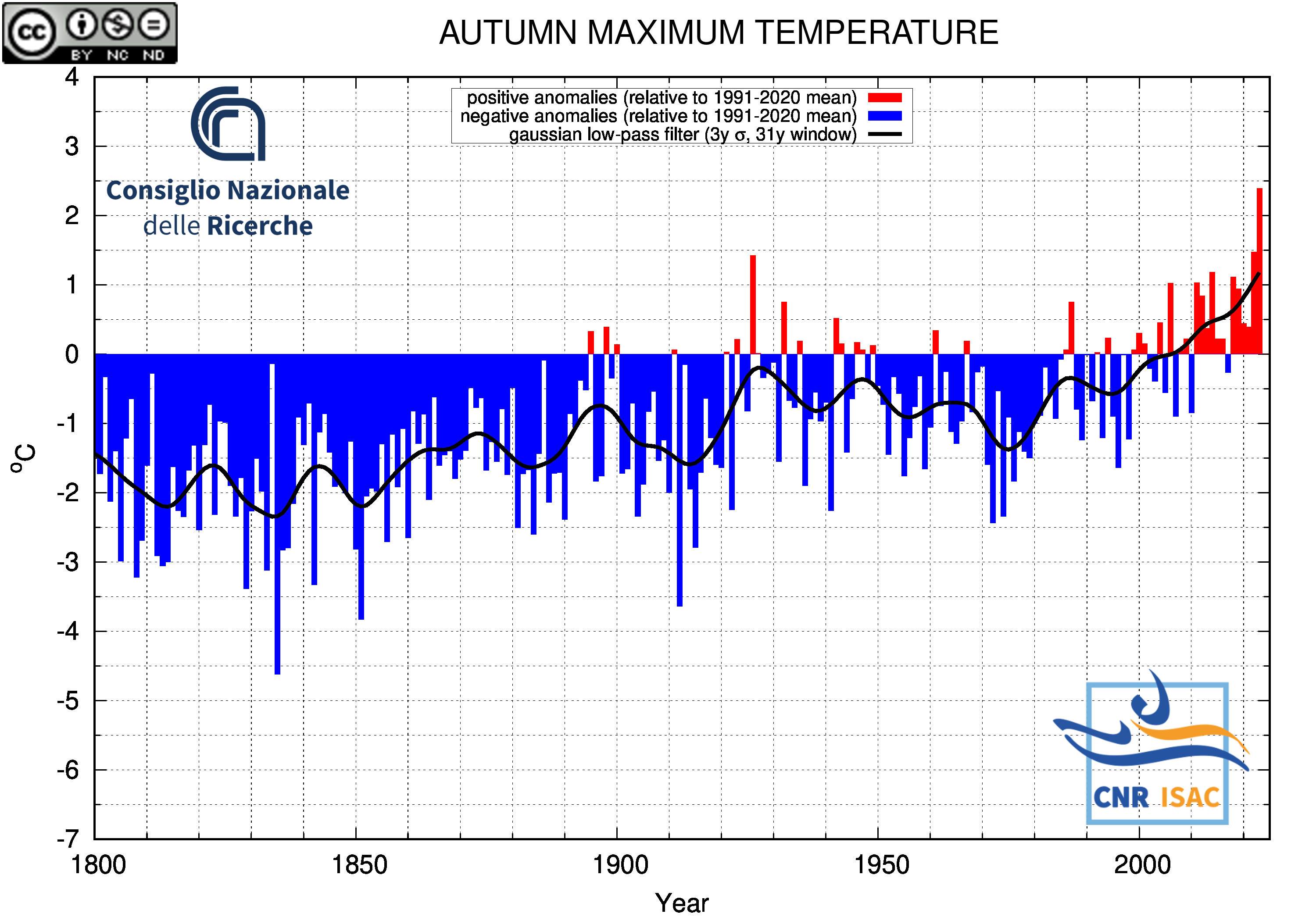
AUTUMN
(SON)
|
TEMPERATURE ANOMALY
|
PRECIPITATION ANOMALY
|
Minimum Temperature
|
Mean Temperature
|
Maximum Temperature
|
|

|
Back to Top
|
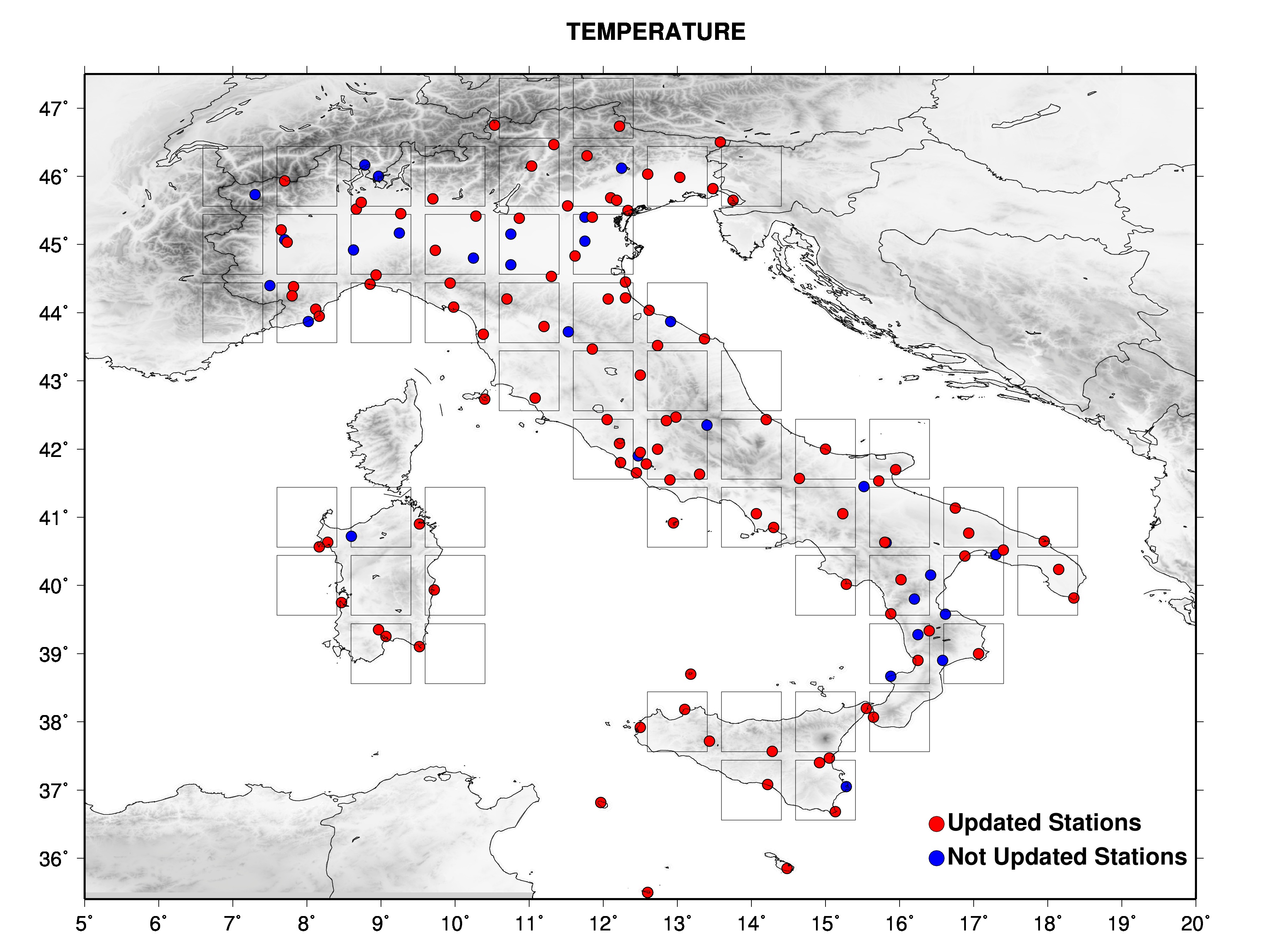
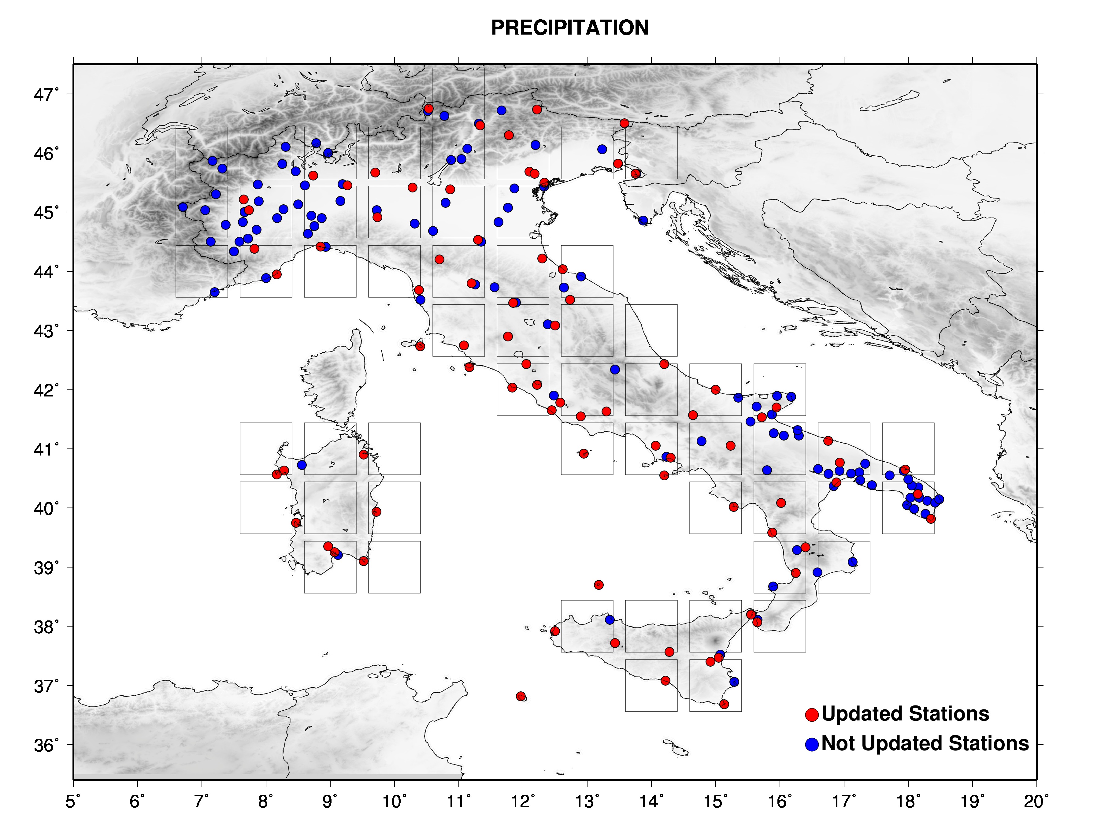
THE DATA SET
The data used to produce the climate bulletins consists of a data set of secular records, coming from the historical Italian
Meteorological Observatories, set up in Brunetti et al (2006)
updated with data from the Global Surface Summery of Day (GSOD), which comprises Italian Air Force and ENAV station data.
At present day, many of the historical Italian Meteorological Observatories are closed and for those still working it is
difficult to obtain data in an automatic and near real time way.
For this reason, the historical Observatories records, when possible, were merged with the modern Air Force network to get a series
wich is updatable in near real time and automatically via GSOD Network managed by NCDC/NOAA.
The whole data set (both merged and not merged series) has been homogenized with statistical techniques to eliminate all
the non-climatic signals due to station history (changes in the instruments, instruments/station relocation, changes in
the observations riles, and so on). See Brunetti et al. (2006)
for details about data homogenization and Venema et al. (2012)
for details about the performances of the mostly used homogenization techniques.
The homogenization is a necessary step to provide time series with a long-term signal as close as possible to the real climate signal.
The figures show the data set with different symbols for stations wich are updated in near real time and stations not updated.
|
CONVERSION INTO ANOMALIES
Stations are located at different elevations and absolute temperature and precipitation
values present strong spatial gradients. For this reason, changes in data availability
can lead to biases when averaging among station series of different length.
An example: if we average the temperature records of three stations with different
mean temperature values (e.g. one station located at sea leve, one at 1000m asl
and the third one at 2000m asl) and with station records having different lengths,
the resulting average series will be positively biased when the coldest station
has no data and negatively biased when the warmest station has no data.
To avoid biases that could result from these problems, monthly temperature and
precipitation series are reduced to anomalies (deviation from the mean for
temperature and ratio for precipitation) from the period with best coverage (1991-2020).
Because many stations do not have complete records for the 1991-2020 period, a gap-filling
technique have been developed to estimate 1991-2020 averages from neighbouring records
(see Brunetti et al., 2006).
The station records converted into anomalies are then interpolated onto a regular grid.
|
GRIDDING METHOD
The grid has one degree resolution, both in latitude and in longitude,
and was realised with an interpolation technique based on a radial weight and an
angular term.
The radial term was realised with a gaussian weighting function with the following form:
with

where i runs along the stations and  is the distance between the station i and the grid point (x,y).
With this choice of the c parameter, we have weights of 0.5 for station
distances equal to 1/4
is the distance between the station i and the grid point (x,y).
With this choice of the c parameter, we have weights of 0.5 for station
distances equal to 1/4  from the grid point
we want to calculate. from the grid point
we want to calculate.
is defined as the mean distance of one grid
point from its next one obtained by increasing both longitude and latitude by one
grid step (it is a sort of mean length of the grid mesh diagonal).
For a grid resolution of 1 deg (as in this case) the
parameter is about 130 km.
The angular term accounts for the geographical separation among the sites
with available time series. It has the following form:

where  is the angular separation
of stations i and l with the vertex of the angle defined at grid point (x,y). is the angular separation
of stations i and l with the vertex of the angle defined at grid point (x,y).
The final weight is the product of the radial and the angular terms.
Each grid point was calculated under one of the following conditions:
i) a minimum of two stations at a distance lower than ,
or ii) a minimum of one station at a distance lower than  .
The grid value computation (once the above conditions were satisfied)
was then performed by considering all stations within a distance of
. .
The grid value computation (once the above conditions were satisfied)
was then performed by considering all stations within a distance of
.
|
THE NATIONAL MEAN SERIES
The national mean seires were obtained by averaging all grid boxes over the italian territory
and not the station anomalies.
The reason is as follows:
The availability of station data is typically not sufficient to ensure an even distribution of
stations throughout a network. But by averaging station anomalies within regions of similar
size (grid boxes) and then calculating the average of all the grid box averages, a more
representative region-wide anomaly can be calculated.
This makes grid box averaging superior to simply taking the average of all stations in the domain.
A network of 1000 stations could theoretically have 700 stations in the northern half of the domain
and 300 stations in the southern half. A simple average of the stations could easily create a bias
in the domain-wide average to those stations in the north.
|
REFERENCES
M. Brunetti, M. Maugeri, F. Monti, T. Nanni; 2006. Temperature and precipitation variability in Italy in the last two centuries from homogenized instrumental time series. International Journal of Climatology, 26, 345-381.
Venema V. K. C., O. Mestre, E. Aguilar, I. Auer, J. A. Guijarro, P. Domonkos, G. Vertacnik, T. Szentimrey, P. Stepanek, P. Zahradnicek, J. Viarre, G. Müller-Westermeier, M. Lakatos, C. N. Williams, M. J. Menne, R. Lindau, D. Rasol, E. Rustemeier, K. Kolokythas, T. Marinova, L. Andresen, F. Acquaotta, S. Fratianni, S. Cheval, M. Klancar, M. Brunetti, C. Gruber, M. Prohom Duran, T. Likso, P. Esteban, and T. Brandsma; 2012. Benchmarking homogenization algorithms for monthly data. Climate of the Past, 8, 89-115, doi:10.5194/cp-8-89-2012.
|
|
Back to Top
|